
Geometric Interpretation#
Introduction#
Vectors as arrows#
To a physicist (or many engineers), vectors (sometimes called Euclidean vectors) are quantities that have both a magnitude (i.e a size) and a direction. They can often be represented by arrows in diagrams or plots, and arise naturally in many areas of physics and engineering. One example is the travel between two points in space, which can easily be represented by vectors.
Vectors as coordinates#
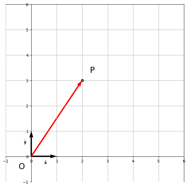
It is convenient to be able to represent vectors in a coordinate system, so that we can perform calculations on them. For example, if we have a coordinate system with an origin \(\mathrm{O}\) and two axes (i.e. orthogonal lines passing through \(\mathrm{O}\)), \(X\) and \(Y\), we can represent the vector \(\mathbf{v}\) as the coordinates of the point \(P\) in the coordinate system. The coordinates of \(P\) are given by the shortest distance from P to the axes. Given these distances, we can write the vector \(\mathbf{v}\) as a linear combination of the two axis vectors:
where \(a\) and \(b\) are the distances from the point \(P\) to the axes, and \(\hat{\mathbf{x}}\) and \(\hat{\mathbf{y}}\) are the “unit” vectors in the \(x\) and \(y\) directions , that is arrows defined to be of unit length and aligned with the two axes. This is known as the geometric interpretation of a vector, and defines a Cartesian coordinate frame.
Of note, if we haven’t already defined a coordinate system, then we can pick one by choosing any point as the origin, \(\mathrm{O}\) and arbitrarily drawing a line through it to represent the \(x\)-axis. The \(y\)-axis can then be defined by the orthogonality condition, i.e. the unique line such that the angle between the two axes is 90 degrees. Picking different choice of axes will give different coordinates for the same vector, but the vector (i.e. arrow) itself is unchanged. This is known as a coordinate transformation.
In 3D, the same process will work, but by measuring distances to planes instead of lines. In this case, we can represent the vector \(\mathbf{v}\) as a linear combination of three axis vectors:
Vectors as columns of numbers#
It is common to write our vector \(a\mathbf{x} + b\mathbf{j}\) in the form
i.e. as a rank 2 column vector in 2D or
for three-dimensions. We’ll eventually see this is equivalent to a matrix with a column rank of 1. The choice to use a column vector rather than a row vector is arbitrary, but it is common to use column vectors in mathematics and physics, while row vectors are more common in computer science. The choice of notation is not important, as long as we are consistent, but we will sometimes want to distinguish between the two. In this case (and this material), we will use the notation \(\mathbf{v}\) for column vectors and \(\mathbf{v}^T\) for row vectors,
To return to a geometric interpretation , we view the first component as the number of units in the direction of the \(x\)-axis and the second component is the number of units in the direction of the \(y\)-axis and so on.
Basic Operations on Vectors#
Based on our intuitive understanding of geometry in the plane, and in 3D, we can define the following operations on pairs of vectors, \(\mathbf{v} = \begin{bmatrix} a \\ b \\ c \end{bmatrix}\) and \(\mathbf{w} = \begin{bmatrix} d \\ e \\ f \end{bmatrix}\):
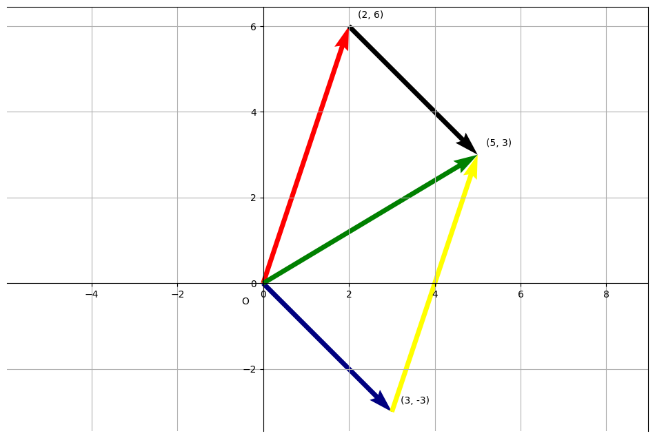
Addition: \(\mathbf{v} + \mathbf{w} = \begin{bmatrix} a \\ b \\ c\end{bmatrix} + \begin{bmatrix} d \\ e \\ f \end{bmatrix} = \begin{bmatrix} a + d \\ b + e \\ c + f \end{bmatrix}\)
Scalar multiplication: \(k\mathbf{v} = k\begin{bmatrix} a \\ b \\ c \end{bmatrix} = \begin{bmatrix} ka \\ kb \\ kc \end{bmatrix}\)
Subtraction: \(\mathbf{v} - \mathbf{w} = \begin{bmatrix} a \\ b \\ c \end{bmatrix} - \begin{bmatrix} d \\ e \\ f \end{bmatrix} = \begin{bmatrix} a - d \\ b - e \\ c - f \end{bmatrix}\). This is equivalent to \(\mathbf{v} + (-1)\mathbf{w}\).
Dot product or inner product: \(\mathbf{v} \cdot \mathbf{w} = ac + bd\) or generally, \(\mathbf{v} \cdot \mathbf{w} = \sum_{i=1}^{n} v_iw_i\)
Cross product: \(\mathbf{v} \times \mathbf{w} = \begin{bmatrix} b \\ c \\ d \end{bmatrix} \times \begin{bmatrix} e \\ f \\ g \end{bmatrix} = \begin{bmatrix} bf - ce \\ cd - af \\ ae - bd \end{bmatrix}\).
More on the dot product#
Geometrically dot product measures the projection of one vector onto the other, and is a measure of how much one vector points in the direction of the other. For example, if \(\mathbf{v} \cdot \mathbf{w} = 0\), then the two vectors are orthogonal or perpendicular to each other, while if \(\mathbf{v} \cdot \mathbf{w} > 0\), then the two vectors are pointing in the same direction, and if we take a dot product with the unit vector in the \(x\)-direction, we get back the \(x\)-component of the vector.
By Pythagoras’ theorem, the magnitude of a vector \(\mathbf{v} = \begin{bmatrix} a \\ b \end{bmatrix}\) is given by \(\|\mathbf{v}\| = \sqrt{a^2 + b^2}\) in 2D, or \(\sqrt\left(\sum\right)_i v_i\) in general, and by the definition of the dot product, we can write this as \(\|\mathbf{v}\| = \sqrt{\mathbf{v} \cdot \mathbf{v}}\). We can also define the angle between two vectors \(\mathbf{v}\) and \(\mathbf{w}\) as \(\cos\theta = \frac{\mathbf{v} \cdot \mathbf{w}}{\|\mathbf{v}\|\|\mathbf{w}\|}\), by considering the triangle formed by the two vectors and the vector between their tips.
More on the cross product#
The cross product is only properly defined in 3D, however it is common to extend the definition to 2D by adding a third component with value 0 to each vector (ie. embedding them on the x-y plane in 3D space). By comstruction, the cross product will be zero in the first two dimensions in this case, so we often only consider the third component.
In general, the cross product is a vector that is orthogonal to both \(\mathbf{v}\) and \(\mathbf{w}\), and has a magnitude equal to the area of the parallelogram formed by the two vectors. The direction of the cross product is given by the right-hand rule, i.e. if you point your fingers in the direction of \(\mathbf{v}\) and curl them towards \(\mathbf{w}\), your thumb will point in the direction of the cross product.
Exercises#
Let’s define \(\mathbf{v} = \begin{bmatrix} 1 \\ 2 \\ 3 \end{bmatrix}\) and \(\mathbf{w} = \begin{bmatrix} 4 \\ 5 \\ 6 \end{bmatrix}\).
What is \(\mathbf{v} + \mathbf{w}\)?
What is \(\mathbf{v} - \mathbf{w}\)?
What is \(2\mathbf{v} + 3\mathbf{w}\)?
Answer
If \(\mathbf{v} = \begin{bmatrix} 1 \\ 2 \\ 3 \end{bmatrix}\) and \(\mathbf{w} = \begin{bmatrix} 4 \\ 5 \\ 6 \end{bmatrix}\), what is \(\mathbf{v} \cdot \mathbf{w}\)? What is \(\|\mathbf{v}\|\)? What is the angle between the two vectors?