Definition#

The classical definition of the derivative of a function $f$ at a point $x_0$ is of given by:

To find the 1st derivative, you will differentiate a function once. To find the 2nd derivative, you will differentiate a function twice. While for many functions, there are analytical solutions, there are also many important functions that do not have analytical solutions. However, finding the differentiation of these function could be important for studying the change of these functions, so numerical differentiation is neccesary.

There are several different ways that numerical differentiation can be done, and each with their merits and demerits. Higher order accuracy in the numerical differentiation would require more sophisticated methods of numerical differentiation.

One of the popular ways to do numerical differentiation is through finite difference. To evaluate the derivative at a point termed $x_0$, the finite difference method uses point or points around the point $x_0$ to find the derivative at the point $x_0$.

Forward difference method (FDM)#

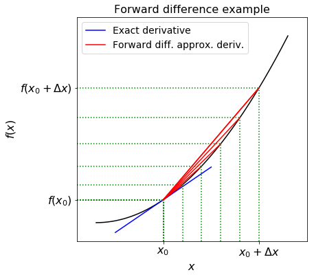
The forward difference is a method of finding the derivative at a point. The forward difference works by taking the gradient between a point $x_0$ and a point in front of $x_0$. As the point in front of $x_0$ becomes closer and closer to $x_0$, then the gradient between $x_0$ and the point in front of $x_0$ becomes closer and closer to the derivative of the function at $x_0$. Because this method uses a point in front of $x_0$, it has forward in its name, and because it uses the difference between $x_0$ and the point in front of $x_0$, it has difference in its name.

For example, we can turn the formal definition of a derivative given above into an approximation rule by replacing the limit as $h$ approaches zero (i.e. the ${\text{lim}}_{h\to \mathrm{\infty }}$) with a small but finite $\mathrm{\Delta }x$ value:

Since this approximate gradient method uses values of $x$ greater than $x_0$ ($\mathrm{\Delta }x>0$), this algorithm is known as the forward difference method.

The figure below illustrates this approximation.

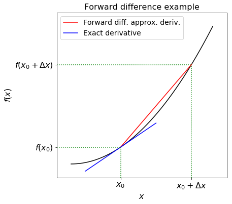
In the figure the derivative is approximated by the slope of the red line, while the true derivative is the slope of the blue line - if the second (and/or higher) derivative of the function is large then this approximation might not be very good, unless you make $\mathrm{\Delta }x$ very small:

dx = 2.37-2.36
df = (0.86289-0.85866)/dx
print("Derivative with FDM = %.5f. " % df)

Estimating accuracy#

As previously discussed, there are many different methods that are possible to use for numerical differentiation. Ultimately, all methods will move closer to the derivative of the function at the point $x_0$ as the $\mathrm{\Delta }x$ used becomes smaller and smaller. What differentiates a good method from a bad method is how accurate the estimate for the derivative is, given that all methods have the same $\mathrm{\Delta }x$ in their equation. Thus what makes a method good/bad is the accuracy of the method.

We can use a Taylor series expansion, or Taylor series analysis, to estimate the accuracy of the method. Recall that Taylor series in one dimension tells us that we can approximate the value of the function at a location in terms of its value, and value of its derivative, at a nearby point -

where $\mathcal{O}(h^3)$ represents the collection of terms that are third-order in $h$ or higher. We call this the Taylor series expansion about (or around) the point $x_0$ (since all the functions in the expansion on the RHS are evaluated at this point). An equivalent way of writing this expansion would be (just define $x$ to be $x_0+h$)

The error increases if $\mathrm{\Delta }x$ increase, while the error decreases if the $\mathrm{\Delta }x$ decreases.

1st order accuracy means that the error and $\mathrm{\Delta }x$ are in a linear relationship. As we make the spacing smaller we expect the error in our derivative to fall linearly, meaning that if we made the spacing 2 times smaller, the error becomes 2 times smaller.

Central difference method (CDM)#

In an attempt to derive a more accurate method we use two Taylor series expansions - one in the positive and one in negative $x$ direction from $x_0$. Since we hope to achieve better than first-order accuracy, we include an extra term in the series:

Using the fact that $(-\mathrm{\Delta }x{)}^2=\mathrm{\Delta }{x}^2$ and the absolute value signs from the definition of $\mathcal{O}$):

Remember that we are looking for an expression for $f^{\prime }(x_0)$. Noticing the sign change between the derivative terms in the two equations, we subtract the second equation from the first to give:

Finally, we can rearrange to get an expression for $f^{\prime }(x_0)$:

which, contrary to the 1st order FDM, is an approximation to the derivative that is 2nd order accurate.

By considering an interval symmetric about $x_0$, we have created a second-order approximation for the derivative of $f$. This symmetry gives the scheme its name - the central difference method.

The figure below illustrates this scheme:

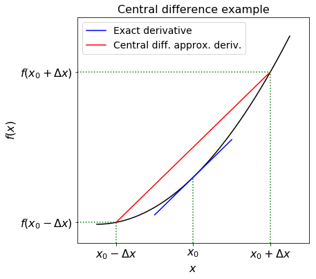
The derivative is approximated by the slope of the red line, while the true derivative is the slope of the blue line. Even without the analysis above it’s hopefully clear visually why this should in general give a lower error than the forward difference. If we halve $h$, the error should drop by a factor of 4, rather than 2 in case of 1st order scheme.

dx = 0.1
df = (0.192916-0.078348)/(2*dx)
print("Derivative with CDM = %.5f. " % df)

dx = 0.08
ddf = (0.339596 - 2*0.367879 + 0.398519)/(dx*dx)
print("2nd Derivative with CDM = %.5f. " % ddf)

Solving differential equations#

One of the most important applications of numerical mathematics in the sciences is the numerical solution of ordinary differential equations (ODEs). While the ODEs you will encounter during your mathematics modules are mostly solvable through analytical solutions, real world ODE are often in the form where it has been proven that no analytical solutions exists. However, many of these ODEs govern important physical processes, and thus, numerical solutions were found for these ODEs.

To recap through an example, suppose we have the general first-order ODE:

That is, the derivative of $u$ with respect to $t$ is some known function of $u$ and $t$, and we also know the initial condition of $u$ at some initial time $t_0$.

If we manage to solve this equation analytically, the solution will be a function $u(t)$ which is defined for every $t>t_0$. Our objective is to find an approximate solution to the ODE at a finite set of points. In this case, we will attempt to find approximate solutions at $t=t_0,$, $t_0+\mathrm{\Delta }t$, $t_0+2\mathrm{\Delta }t$, $t_0+3\mathrm{\Delta }t$, $\dots$.

It is frequently useful to think of the independent variable, $t$, as representing time. A numerical method steps forward in time units of $\mathrm{\Delta }t$, attempting to calculate $u(t+\mathrm{\Delta }t)$ in using the previously calculated value $u(t)$.

More on timestepping an ODE can be found here.

Exercises#

import numpy as np
import matplotlib.pyplot as plt

def diff(f, x, dx=1e-6):
    numerator = f(x + dx) - f(x - dx)
    derivative = numerator / ( 2.0 * dx )
    return derivative

dx = 0.01
x = 0
f = np.exp
derivative = diff(f, x, dx)
print("The approximate derivative of exp(x) at x = 0 is: %f. The error is %f."
      % (derivative, abs(derivative - 1)))
x = 0

def g(x):
    return np.exp(-2*x)

derivative = diff(g, x, dx)
print('The approximate derivative of exp(-2*x) at x = 0 is: {0:.5f}.  The error is {1:.5f}.'
        .format(derivative, abs(derivative - (-2.0))))

x = 2*np.pi
f = np.cos
derivative = diff(f, x, dx)
print('The approximate derivative of cos(x) at x = 2*pi is: {0:.5f}.  The error is {1:.5f}.'
        .format(derivative, abs(derivative - 0)))

x = 1
f = np.log
derivative = diff(f, x, dx)
print('The approximate derivative of ln(x) at x = 0 is: {0:.5f}.  The error is {1:.5f}.'
        .format(derivative, abs(derivative - 1)))

The approximate derivative of exp(x) at x = 0 is: 1.000017. The error is 0.000017.
The approximate derivative of exp(-2*x) at x = 0 is: -2.00013.  The error is 0.00013.
The approximate derivative of cos(x) at x = 2*pi is: 0.00000.  The error is 0.00000.
The approximate derivative of ln(x) at x = 0 is: 1.00003.  The error is 0.00003.

Derivative of $sin(x)$#

We will compute

$$\frac{d(\sin x)}{dx}\text{at}x=0.8$$

using FDM and CDM. We will evaluate these derivatives for decreasing values of $h$ (starting with $h=1.0$ and halving) and compare the values against the exact solution.

At first let’s define forward_diff and central_diff functions:

def forward_diff(f, x, dx):
    fx = f(x)
    fxph = f(x + dx)
    return (fxph - fx) / dx


def central_diff(f, x, dx):
    fxph = f(x + dx)
    fxnh = f(x - dx)
    return (fxph - fxnh) / (2 * dx)

We know that the exact solution is \(\frac{d \sin(x){dx}=\cos{x}\), we can evaluate that and store to compare later with the numerical solution:

exact = np.cos(0.8)
print("Exact derivative at sin(0.8) = %.5f." % exact)

Exact derivative at sin(0.8) = 0.69671.

Now, we can compute solution with two schemes and compare with the exact solution:

Show code cell source Hide code cell source

# headers for the following errors outputs
print('%20s%40s' % ('Forward differencing', 'Central differencing'))

# We're going to store all the values for plotting,
# initialise variable for these
fd_errors = []
cd_errors = []
dx_all = []
dx = 1.0  # An initial mesh spacing

for i in range(10):
    fd = forward_diff(np.sin, 0.8, dx)
    cd = central_diff(np.sin, 0.8, dx)
    print('%10g (error=%10.2g)         %10g (error=%10.2g)' %
          (fd, abs(fd - exact), cd, abs(cd - exact)))
    # Store the h and the errors
    dx_all.append(dx)
    fd_errors.append(abs(fd - exact))
    cd_errors.append(abs(cd - exact))
    dx = dx / 2  # Halve h for the next iteration

Forward differencing                    Central differencing
  0.256492 (error=      0.44)           0.586258 (error=      0.11)
  0.492404 (error=       0.2)           0.668038 (error=     0.029)
  0.600269 (error=     0.096)           0.689472 (error=    0.0072)
  0.650117 (error=     0.047)           0.694894 (error=    0.0018)
  0.673843 (error=     0.023)           0.696253 (error=   0.00045)
  0.685386 (error=     0.011)           0.696593 (error=   0.00011)
  0.691074 (error=    0.0056)           0.696678 (error=   2.8e-05)
  0.693897 (error=    0.0028)             0.6967 (error=   7.1e-06)
  0.695304 (error=    0.0014)           0.696705 (error=   1.8e-06)
  0.696006 (error=    0.0007)           0.696706 (error=   4.4e-07)

Let’s plot the errors in a log-log plot so that we can see the relationship between the error and the increment:

Show code cell source Hide code cell source

# Set up figure
fig = plt.figure(figsize=(7, 5))
ax1 = plt.subplot(111)

ax1.loglog(dx_all, fd_errors, 'b.-', label='Forward diff.')
ax1.loglog(dx_all, cd_errors, 'k.-', label='Central diff.')
ax1.set_xlabel('$\Delta x$', fontsize=16)
ax1.set_ylabel('Error', fontsize=16)
ax1.set_title('Convergence plot', fontsize=16)
ax1.grid(True)
ax1.legend(loc='best', fontsize=14)

plt.show()

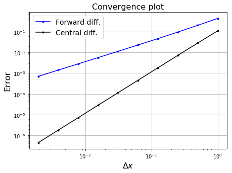
The errors fall linearly in $\mathrm{\Delta }x$ on a log-log plot, therefore they have a polynomial relationship. The slopes of the lines indicate the order of the relationship - slope 1 for forward difference and slope 2 for central difference.