Transforming inhomogeneous BCs to homogeneous#

Consider a general 1 + 1 dimensional heat equation with inhomogeneous boundary conditions:

For separation of variables to be successful, we need to transform the boundary conditions to homogeneous ones. We do that by seeking the solution of the form $u(x,t)=U(x,t)+S(x,t)$ where $S$ is of the form

and $A(t),B(t)$ are unknown functions chosen such that $S(t,x)$ satisfies the original boundary conditions

or after substituting in $S$:

This is a simple system of two linear equations for $A$ and $B$ which we can solve using Cramer’s rule. Substituting $u=U+S$ in the original PDE, we get, in general, an inhomogeneous PDE

but the boundary conditions are now homogeneous

and the initial condition becomes

Example#

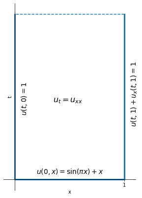
Let us solve the initial-boundary-value problem (Farlow 1993, p.47 problem 1):

where $u\equiv u(t,x)$ is temperature in the domain. For simplicity let us choose $k^2=1$. Note that mathematically it doesn’t really matter what $k^2$ is since we can always transform $u$ such that $k^2$ is unity (in engineering it, of course, matters).

Let us draw a simple diagram to visualise our domain and auxiliary conditions.

Show code cell source Hide code cell source

import matplotlib.pyplot as plt


fig = plt.figure(figsize=(5, 7))
ax = fig.add_subplot(111)

ax.plot([0, 0, 1, 1], [1.5, 0, 0, 1.5], 'C0', linewidth=3)
ax.plot([1, 0], [1.5, 1.5], '--', c='C0')
ax.text(0.2, 0.05, r'$u(0,x) = \sin (\pi x) + x$', fontsize=14)
ax.text(0.05, 0.6, r'$u(t, 0) = 1$', rotation=90, fontsize=14)
ax.text(1.05, 0.5, r'$u(t, 1) + u_x(t,1)= 1$', rotation=90, fontsize=14)
ax.text(0.35, 0.7, r'$u_t = u_{xx}$', fontsize=16)

ax.set_xlim(-0.1, 1.1)
ax.set_ylim(-0.1, 1.6)

ax.set_aspect('equal')
ax.set_xlabel('x')
ax.set_ylabel('t')
ax.spines['left'].set_position('zero')
ax.spines['bottom'].set_position('zero')
ax.spines['right'].set_visible(False)
ax.spines['top'].set_visible(False)
ax.set_xticks([1])
ax.set_yticks([])

plt.show()

First we have to transform the BCs to homogeneous ones. Looking at BCs, we could guess that we only need to translate $u$ by $+1$, i.e. $u=U+S=1$ BC will become homogeneous for $U$. But we can follow the above procedure and get $A=B=1$. Then $S=1-x/L+x/L=1$. So our transformation is, as we expected,

Substituting this in the original problem we get the transformed problem

which we can now solve using separation of variables. We seek solutions of the form $U=X(x)T(t)$ and substitute it into our PDE and divide both sides by $XT$ to get separated variables:

where LHS depends only on $t$ and RHS on $x$. Since $x,t$ are independent of each other, each side must be a constant, say $\alpha$. We get two ODEs:

Now notice that $\alpha$ must be negative, i.e. $\alpha =-{\lambda }^2$ since then $T^{\prime }=-{\lambda }^{2}T$ has the solution $T(t)=C\exp (-{\lambda }^{2}t)$ which decays with time, as it should (instead of growing to $\mathrm{\infty }$). Then $X(x)=D\sin (\lambda x)+E\cos (\lambda x)$ and multiplying them together:

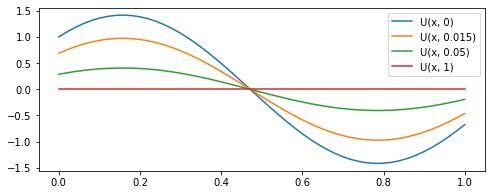
where $D,E$ are arbitrary constants (multiplying them by $C$, another constant, doesn’t matter). We now have infinitely many simple solutions to $u_t=u_{xx}$. Solutions are simple because any temperature $u(x,t)$ will have the same “shape” for any value of $t$, but it exponentially decays with time.

Show code cell source Hide code cell source

import numpy as np


xx = np.linspace(0, 1, 51)
tt = [0, 0.015, 0.05, 1]

fig = plt.figure(figsize=(8, 3))
ax = fig.add_subplot(111)

for t in tt:
    U = np.exp(-25*t) * (np.sin(5*xx) + np.cos(5*xx))
    ax.plot(xx, U, label=f'U(x, {t})')

ax.legend(loc='best')
plt.show()

However, as we can see from the figure above, not all of these solutions satisfy auxiliary conditions, but some of them do and we are only interested in the ones which do. So we substitute $U$ in BCs:

where we choose $D\ne 0$ as we are interested in non-trivial solutions, so we have $\sin \lambda +\lambda \cos \lambda =0$.

Show code cell source Hide code cell source

x = np.linspace(-4, 15, 501)

fig = plt.figure(figsize=(10, 5))
ax = fig.add_subplot(111)

ax.plot(x, np.sin(x) + x*np.cos(x), label=r'$y = \sin \lambda + \lambda \cos \lambda$')

ax.legend(loc='best')
ax.set_xlim(-3, 12)
ax.set_ylim(-12, 10)
ax.set_xlabel(r'$\lambda$')
ax.spines['left'].set_position('zero')
ax.spines['bottom'].set_position('zero')
ax.spines['right'].set_visible(False)
ax.spines['top'].set_visible(False)
ax.set_yticks([])
plt.show()

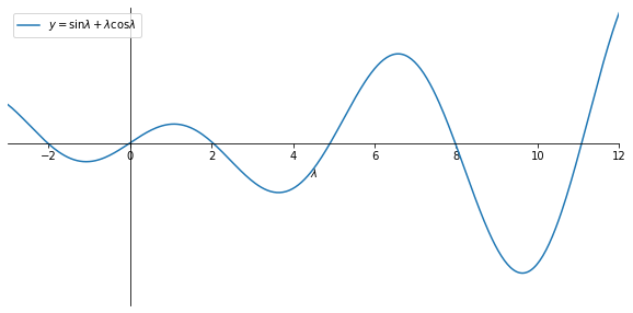
We have to find the roots numerically, which we do below.

# find roots of f(x) = sinx + x cosx = 0
    
from scipy.optimize import fsolve

def f(x): 
    return np.sin(x) + x*np.cos(x)

# the list are initial guesses which we approximate from the graphs above
lambdas = fsolve(f, [2, 5, 8, 11, 14])
for i in range(len(lambdas)):
    print(f'lambda {i+1} = {lambdas[i]}')

lambda 1 = 2.0287578379859226
lambda 2 = 4.913180439951472
lambda 3 = 7.978665712411702
lambda 4 = 11.085538406152708
lambda 5 = 14.207436725344412

Also note that we may only consider positive roots $\lambda$ because $\sin \lambda +\lambda \cos \lambda =\sin (-\lambda )+(-\lambda )\cos (-\lambda )$.

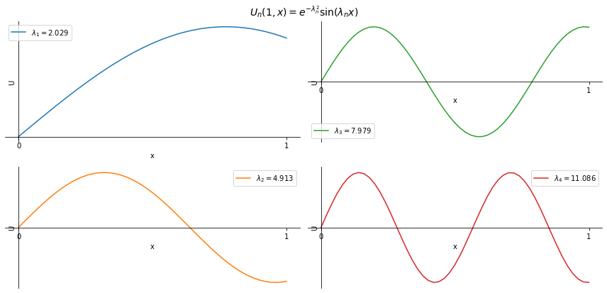
There are infinitely many roots ${\lambda }_i$, which we call the eigenvalues, so we have infinitely many solutions

and multiplying them together we get the eigenfunctions:

Each one of these eigenfunctions satisfies the PDE and the BCs.

fig, ax = plt.subplots(2, 2, figsize=(12, 6))
ax = ax.flatten(order='F')

for i, lam in enumerate(lambdas[:-1]):
    U = np.exp(-lam**2) * np.sin(lam*xx)
    ax[i].plot(xx, U, c=f'C{i}', label=fr'$\lambda_{i+1} = {lam:.3f}$')

    ax[i].legend(loc='best')
    ax[i].set_xlabel('x')
    ax[i].set_ylabel('U')
    ax[i].spines['left'].set_position('zero')
    ax[i].spines['bottom'].set_position('zero')
    ax[i].spines['right'].set_visible(False)
    ax[i].spines['top'].set_visible(False)
    ax[i].set_xticks([0, 1])
    ax[i].set_yticks([])
    
fig.suptitle(r'$U_n(1, x) = e^{-\lambda_n^2} \sin (\lambda_n x)$', fontsize=14)

plt.tight_layout(rect=[0, 0.03, 1, 0.95])
plt.show()

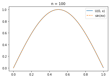
But we still need to satisfy the initial condition. Let us assume that we could do that by summing up all functions $U_n$ (which we are allowed to do because of linearity). That is, consider a Fourier series of the eigenfunctions:

where we want to choose coefficients $D_n$ such that the initial condition $U(0,x)=\sin (\pi x)$ is satisfied:

To find the coefficients $D_n$ we multiply both sides by $\sin ({\lambda }_{n}x)$ and integrate from $0$ to $1$:

and solve for $D_n$:

Show code cell source Hide code cell source

x = np.linspace(0, 1, 201)
x0 = [2 + k*np.pi for k in np.arange(100)]  # initial guesses

lambdas = fsolve(f, x0)

U = 0
for i, lam in enumerate(lambdas, 1):
    q1 = np.pi*np.sin(lam) / (np.pi**2 - lam**2)  # numerator
    q2 = 0.5 - np.sin(2*lam) / (4*lam)  # denominator
    D = q1/q2
    
    if i < 7:
        print(f'D_{i} = {D}')
    
    U += D*np.sin(lam*x)
    
plt.plot(x, U, label='U(0, x)')
plt.plot(x, np.sin(np.pi*x), '--', label=r'$\sin (\pi x)$')
plt.legend(loc='best')
plt.title('n = 100')
plt.show()

D_1 = 0.81933447202856
D_2 = 0.4149624369818997
D_3 = -0.11413858717466217
D_4 = 0.054925619476512
D_5 = -0.03248712860366395
D_6 = 0.02150824645327097

And now $U$ satisfies the PDE, BCs and IC. So our solution $u=U+S$ is

where ${\lambda }_n$ and $D_n$ are given above.